Big Wins
The Guinness world record for the most massive single win at an online slot machine is held by the British ex-soldier Jon Heywood, who won roughly £ 13.2 million after a 25p bet playing online casino on Betway. That’s a staggering 52 000 000x return on one single bet. On this occasion the record was set on the popular Mega Moolah slot – provided by Microgaming. Mega Moolah is a so-called progressive jackpot slot, meaning a small percentage of every bet goes towards an individual jackpot contribution that gets released once in a blue moon to a very lucky gambler. That’s what enables these types of games to have potential returns of millions in one single bet
Traditional slot games that are even more popular than abovementioned jackpot games, for example, Starburst – provided by Netent, and Book o Dead – supplied by Play’n GO, offer maximum payouts in the interval of 500 – 5 000x return on a single bet depending on the volatility of the game. Not as extreme as the jackpot games since there is no jackpot contribution, but still potentially very rewarding for the player.
Random walk
Readers familiar with the literature on finance and investing will recognize that the title of this article was borrowed from one of the classic books on investing – A Random Walk Down Wall Street, by Burton G. Malkiel. Mr. Maikel argues that the movement of stock prices are completely random and non-predictable.
“The past history of stock prices cannot be used to predict the future in any meaningful way.”
There are different types of random walks:
- Real random walk without a trend implies, in a time-series dataset, that a value at time T+1 (Next observation) will be equal to the value of the current observation (T) + a random, independent, error component. In other words, the next value in the dataset is impossible to predict.
- Non-mean-reverting random walk has a drift variable added to the previous observation and the error component. If the drift variable is >0, the random walk will drift upwards (positive).
Numbers
Enough of finance talk, let’s get into the numbers for our slot machine!
The expected value of each spin is calculated as follows: Bet Amount x RTP (the return to player). This information is available for most of the slot games out there for regulatory reasons.
In our example, we will use data from the slot game Mystic mirror by Red Rake Gaming. Mystic Mirror has, according to the game developer, a theoretical Return To Players of 95.2%, i.e., for every C$ 5 bet on the slot game, a player can expect to receive C$ 4.76 back.
The formula to calculate the standard deviation of the game is more complicated and requires an ample sample size of data (real previously played spins) to make a good estimation. We want to point out that it is an estimation because only the game developer will know the actual game mechanics. This information is not shared with the public since it is considered a “trade secret” among the game providers. With that said, due to the size of the observations from real casino games, our estimation will be very close to the actual value, especially on the more frequent payouts. More info about this later.
For us to calculate the standard deviation of a slot machine, we need to understand that the payout structure of a slot machine is like the payout structure for a lottery. Imagine a simple lottery with only two payouts:
51% of the times a player will lose the amount staked (payout = 0 x)
49% of the times a player will win double the amount staked (payout 2 x)
The expected value of this lottery given a C$ 5 stake amount is 0.51 x 0 + 0.49 x 10 = C$ 4.9. Meaning the house, in this case, has a 2% edge on the player (4.9/5-1 = -0.02)
To calculate the variance and standard deviation of this lottery we square the value of the difference between the payoffs, in the simplified version of the lottery above the two payoffs are 0, and 10, and the expected value (4.9). After that, we sum these values with the probabilities of the events occurring. Finally, to derive the standard deviation, take the square root of the variance value.
From our simplified lottery above we derive at a standard deviation of SQRT((0-4.9)^2*0.51 + (10-4.9)^2*0.49) = C$ 4.999
The calculation is easy to follow because nearly half the times, you will lose C$ 5, and the other half you will win C$ 5.
So now let us look at the estimated payout table for our slot game when playing with a C$ 5 stake:
| Descr | Payout | Frequency |
| 0x | C$ 0 | 71.32% |
| 0.25x | C$ 1.25 | 8.24% |
| 0.5x | C$ 2.5 | 5.87% |
| 0.75x | C$ 3.75 | 4.19% |
| 1.25x | C$ 6.25 | 2.99% |
| 1.5x | C$ 7.5 | 2.13% |
| 1.75x | C$ 8.75 | 1.52% |
| 2x | C$ 10 | 1.08% |
| 2.5x | C$ 12.5 | 0.77% |
| 5x | C$ 25 | 0.55% |
| 6.25x | C$ 31.25 | 0.39% |
| 7.5x | C$ 37.5 | 0.28% |
| 10x | C$ 50 | 0.20% |
| 25x | C$ 125 | 0.14% |
| 26.25x | C$ 131.25 | 0.10% |
| 38x | C$ 190 | 0.07% |
| 68.75x | C$ 343.75 | 0.05% |
| 250.25x | C$ 1251.25 | 0.04% |
| 489.25x | C$ 2446.25 | 0.03% |
| 718.25x | C$ 3591.25 | 0.02% |
| 1200x | C$ 6000 | 0.01% |
| 100.00% |
The data above is from a sample size larger than 200 000 spins. The 21 different payouts included in the table have been observed data points from actual spins. The higher payout frequencies are derived using Excel Solver, from the information of the slot machines RTP, the more frequent payout frequencies and the maximum win. As per Red Rakes gaming information about the slot, we know that the maximum payout from Mystic Mirror is 1200 x the amount staked. In the above case, that is C$ 5 x 1200 =C$ 6000. A lot of money from one single C$ 5 spin!
From the theorem Law of large numbers, we can assume that the above-estimated frequencies on the more frequent payouts, such as 0 x, 0.25 x, 0.5 x and 1.25 x will be very close to their real value. This assumption is especially correct for the times the slot game does not pay back anything from a spin, i.e., the 0 x frequency. In our sample size, this happened 71.3% of the time. Naturally, for the less frequent payouts, such as a 250.25 x win of staked amount, the error margin of the estimate will be higher due to the requirement of a significantly larger sample size for the rare events. The estimated frequencies in the table above, derived from Excel Solver, with the assumption that higher payouts are always rarer. While this generally is true, there will be slot machines that are “fat tailed” on the distribution of the payouts, I.e., some payouts will have a higher probability of occurring then a corresponding probability for a lower payout.
The calculated variance of the 21 pay outs and their corresponding probabilities from the table above equals C$ 9511 or a standard deviation per spin of C$ 97.5 (the square root of the variance).
Simulation
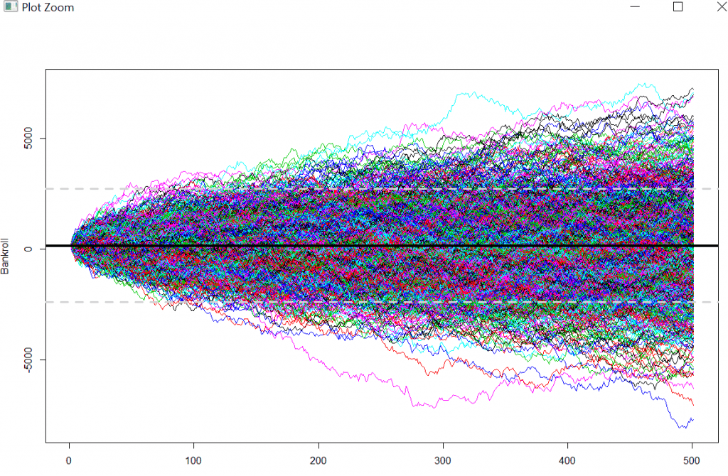
With the information available to us now, the expected value per spin, derived from the RTP %, and the standard deviation per spin, we can generate a simulation of multiple spins and replicate these trials. In other words, a Random walk.
We are going to simulate a scenario where an online casino offers a 100% match up bonus – up to C$ 100 – a common type of bonus offered by Unibet here. Furthermore, we are going to assume a 25x wagering requirement and maximum allowed bet amount per spin to play through the wagering requirement at C$ 5.
The required variables we are using are T = Time or Trial dimension. In terms of time, the number of periods we will run the simulation. Using the example above, we will play 500 Spins betting C$ 5 on every spin. k = How many random walks we will simulate. In our example, we are going to simulate 1000 different random walks; We can think of this as 1000 players playing through the bonus and their outcomes being independent. Initial.value = Will be the starting amount of our bankroll. In this example, we are taking advantage of the full bonus; in other words, we are depositing C$ 100 and receiving another C$ 100, bringing the total to C$ 200.
R code follows below:
#Matplot monte carlo
# Generate k random walks across time {0, 1, … , T}
T <- 500
k <- 1000
initial.value <- 200
GetRandomWalk <- function() {
# Add a standard normal at each step
initial.value + c(0, cumsum(rnorm(T, mean = -0.24, sd = 97.5)))
}
# Matrix of random walks
values <- replicate(k, GetRandomWalk())
Resulting matrix
Running the above code, we have created a matrix (think of it as a table with columns and rows, where every column represents a player, 1000 columns. Every row represents a value of the player’s bankroll after every period, or trial, up to a total of 500 trials.